
Curve fitting demo in
ABC FORTH
Ching-Tang Tseng
2015/4/12 Hamilton , New Zealand
1. Abstract
This article demonstrates it is quite simple to translate a typical traditional BASIC program into ABC FORTH
system. Original program implemented out curve fitting by Lagrange interpolating
polynomial method. A test program, according to the value of the exponential function
to be the input data, could give out all the coefficients of a polynomial by
the specified order.
2. Reference
A BASIC Program
for Exact Curve Fitting
It is often required to find a polynomial to fit
some function for which we know only a few values; the program given here in
figure 1 calculates the coefficients of a polynomial such that the fit is exact
for those data points.
If we have p+1 data points, then a
polynomial of order p (or greater) can be found that will pass
through all of these points (although in some special cases an exact polynomial
of order less than p can be found). The minimum order polynomial
is unique and it is the coefficients of this polynomial that are found by the
program.
The program uses a method based on the Lagrange
interpolating polynomial. For each value of abscissa: xj
( j is an integer: 0
j
p ) we construct a polynomial: Aj (x)
of order p that has the following properties: firstly, it has
unity value at xj and secondly it is zero for all xi
( 0
i
p; i
j ). Aj (x) is
constructed in two steps; firstly, using program statements: 130 - 190, a
polynomial Fj (x) is constructed:
Fj (x) = ( x - x0
)( x - x1 ).......( x - xj-1 )( x - xj+1
)......( x - xp )
this clearly has the second property; by evaluating Fj (x)
at xj (lines 220 - 230) we can find Aj (x)
that has both properties (line 200):
Fj (x)
|
||
Aj (x)
|
=
|
|
Fj ( evaluated at xj )
|
Having calculated an Aj (x)
for all xj , weighting the coefficients of each Aj
(x) by the data value corresponding to xj
and summing the polynomials gives the required function; this is calculated and
printed by statements 275 - 315.
The program given here assumes that the data are
given for values of x = 0,1,2,3.... but appropriate scaling will
allow fitting to any set of equally spaced data (modifications to statement 160
will allow nonuniformly spaced data to be fitted). Although written and tested
on a Hewlett Packard 85 computer all of the statements should be suitable for
other interpreters with little or (in most cases) no modification.
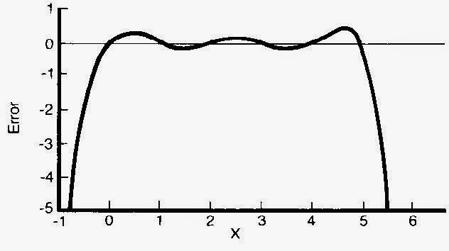
By way of example, a fifth order fit to the
function exp(x) is calculated, for x = 0,1,2,3,4
and 5, giving the coefficients of the required polynomial:
H0 = 1
H1 = 2.74952
H2 = -3.30606
H3 = 3.03500
H4 = -.885002
H5 =.124822
The error (H0 + H1 x
+ H2 x2 + H3 x3 + H4 x4
+ H5 x5 - exp(x)) is plotted in
figure 2; as can be seen the fit is exact at x = 0,1,2,3,4 and 5
and elsewhere the interpolation is good.
Department of Electrical
Figure 1: Program Listing
100 COM A(57,56), C(57), H(56), Z(56)
105 INTEGER I, J, N, N1, P
110 CLEAR
115 LINPUT "Order of fit:",P$ @ P = VAL(P$) @ IF P > 56 THEN BEEP @ GOTO 115
120 GOSUB 245
125 FOR J = 0 TO P
130 GOSUB 235
135 C(0) = 1
140 FOR N = 0 TO P
145 N1 = N + 1
150 IF N = J THEN N = N + 1
155 IF N > P THEN 190
160 B0 = -N
165 FOR I = 1 TO N1
170 A(I,J) = B0 * C(I) + C(I-1)
175 NEXT I
180 A(0,J) = B0 * C(0)
185 FOR I = 0 TO N1 @ C(I) = A(I,J) @ NEXT I
190 NEXT N
195 GOSUB 220
200 FOR I = 0 TO P @ A(I,J) = A(I,J)/C(0) @ NEXT I
205 NEXT J
210 GOSUB 275
215 BEEP 100,190 @ DISP "finished" @ STOP
220 FOR I = P TO 1 STEP -1
225 C(I-1) = C(I) * J+C(I-1) @ NEXT I
230 RETURN
235 FOR I = 0 TO P + 1 @ C(I) = 0 @ NEXT I
240 RETURN
245 PRINT @ PRINT "INPUT DATA" @ PRINT "==========" @ PRINT
250 FOR I = 0 TO P
255 DISP @ DISP "Y value for abscissa value:"; I @ INPUT Z(I)
260 PRINT "Z("; I; ")= "; Z(I)
265 NEXT I
270 RETURN
275 PRINT @ PRINT "POLYNOMIAL FIT" @ PRINT "==============" @ PRINT
280 FOR I = 0 TO P @ H(I) = 0 @ NEXT I
285 FOR J = 0 TO P
290 FOR I = 0 TO P
295 H(I) = Z(J) * A(I,J) + H(I)
300 NEXT I
305 NEXT J
310 FOR I = 0 TO P @ PRINT "H("; I; ")= "; H(I) @ NEXT I
315 RETURN
320 END
NOTES
·
This article was published in ELECTRONIC
ENGINEERING, 57, No 698; FEBRUARY 1985 p 38.
Last
updated: 1 Oct
2005 ; © Lawrence Mayes,
1985/2000-2005
3. Program translated to the ABC FORTH system
\ ABC FORTH demo code:
Lagrange interpolating polynomial curve fitting.
\ Author: Ching-Tang Tseng,
Hamilton, New Zealand
\ Date:2012-08-06(original),
2015-04-09(renewed for posting)
\ Contact:
ilikeforth@gmail.com
\ Reference:
\ Lawrence J. Mayes
ELECTRONIC ENGINEERING, 57, No 698; FEBRUARY 1985 p 38.
\ Description:
\ This program uses a method
based on the Lagrange interpolating polynomial.
\ ZZ(i) is the input raw data
array.
\ Matrix AAA(i,j) is the
difference table manipulation matrix.
\ HH(i) is the output
coefficients array of the fitted polynomial.
\ Remark: Original array and
matrix structures in ABC FORTH system
\ without 0 indexes function.
0 index function to be included
\ after this program could be
implemented out.
5 INTEGERS I J N N1 P
: INPUT-ORDER BASIC
10 PRINT " Order of fit:
"
20 INPUTI P
30 IF P > 56 THEN 50
40 GOTO 70
50 PRINT " Order P cannot
> 56, Re-enter please. "
60 GOTO -10
70 END ;
56 ARRAY ZZ
: SUB245 BASIC
10 RUN INPUT-ORDER
20 PRINT " Input data:
"
30 PRINT " ===========
"
40 FOR I = 0 TO P \ Index start from 0
50 PRINT " Y value for X
abscissa value: " ; I
60 INPUTR ZZ ( I )
70 PRINT " Y( " ; I
; " )=" ; { ZZ ( I ) }
80 NEXT I
90 END ;
57 ARRAY CC
: SUB235 BASIC
10 FOR I = 0 TO P + 1 \ Index is an arithmetical expression
20 LET { CC ( I ) = 0 }
30 NEXT I
40 END ;
56 ARRAY HH
57 56 MATRIX AAA
: SUB275 BASIC
10 PRINT " Polynomial
fit: "
20 PRINT "
=============== "
30 FOR I = 0 TO P
40 LET { HH ( I ) = 0 }
50 NEXT I
60 FOR J = 0 TO P
70 FOR I = 0 TO P
80 LET { HH ( I ) = ZZ ( J )
* AAA ( I J ) + HH ( I ) }
90 NEXT I
100 NEXT J
110 FOR I = 0 TO P
120 PRINT " HH( " ;
I ; " )= " ; { HH ( I ) }
130 NEXT I
140 END ;
INTEGER I-1
: SUB220 BASIC
10 FOR I = P TO 1 STEP -1
20 LET I-1 = I - 1
30 LET { CC ( I-1 ) = CC ( I
) * I>R ( J ) + CC ( I-1 ) }
40 NEXT I
50 END ;
INTEGER Q
REAL B0
: MAIN BASIC
10 RUN SUB245
20 FOR J = 0 TO P
30 RUN SUB235
40 LET { CC ( 0 ) = 1 }
50 FOR N = 0 TO P
60 LET N1 = N + 1
70 IF N = J THEN 90
80 GOTO 100
90 LET N = N + 1
100 IF N > P THEN 200
105 LET Q = NEGATE N
110 LET { B0 = I>R ( Q ) }
120 FOR I = 1 TO N1
130 LET I-1 = I - 1
140 LET { AAA ( I J ) = B0 *
CC ( I ) + CC ( I-1 ) }
150 NEXT I
160 LET { AAA ( 0 J ) = B0 *
CC ( 0 ) }
170 FOR I = 0 TO N1
180 LET { CC ( I ) = AAA ( I
J ) }
190 NEXT I
200 NEXT N
210 RUN SUB220
220 FOR I = 0 TO P
230 LET { AAA ( I J ) = AAA (
I J ) / CC ( 0 ) }
240 NEXT I
250 NEXT J
260 RUN SUB275
270 PRINT "
Finished."
280 END ;
\ Usage:
\ (1) Execute the following
instruction GIVEN first to get the input data.
\ (2) Next, execute MAIN,
then enter the data which you got above and
\ follows the Q & A procedures.
: GIVEN BASIC
10 RUN CR CR
20 FOR I = 0 TO 5
30 PRINT " Y( " ; I
; " )= " ; { EXP ( I>R ( I ) ) }
40 NEXT I
50 RUN CR CR
60 END ;
\S
Execution results:
GIVEN
Y( 0 )= 1.00000000000
Y( 1 )= 2.71828182846
Y( 2 )= 7.38905609893
Y( 3 )= 20.0855369232
Y( 4 )= 54.5981500331
Y( 5 )= 148.413159103
ok
MAIN
Order of fit: ? 5
Input data:
===========
Y value for X abscissa value:
0 ? 1.00000000000
Y( 0 )= 1.00000000000
Y value for X abscissa value:
1 ? 2.71828182846
Y( 1 )= 2.71828182846
Y value for X abscissa value:
2 ? 7.38905609893
Y( 2 )= 7.38905609893
Y value for X abscissa value:
3 ? 20.0855369232
Y( 3 )= 20.0855369232
Y value for X abscissa value:
4 ? 54.5981500331
Y( 4 )= 54.5981500331
Y value for X abscissa value:
5 ? 148.413159103
Y( 5 )= 148.413159103
Polynomial fit:
===============
HH( 0 )= 1.00000000000
HH( 1 )= 2.74952933754
HH( 2 )= -3.30606647675
HH( 3 )= 3.03499879102
HH( 4 )= -.885001709373
HH( 5 )= .124821886021
Finished. ok
**************************************************
Original paper supplied
output result data are:
H0 = 1
H1 = 2.74952
H2 = -3.30606
H3 = 3.03500
H4 = -.885002
H5 = .124822
**************************************************
4. This diagram shows the
error condition in the specified range.

5. All implementation are
finished in Win32Forth V6.14.03 added-in ABC FORTH V659 under W7 operating
system.